Oracles

Oracles are simply boolean functions. We give an input to the function or oracle or black box, and it returns an output, without us knowing its inner workings.

Quantum oracles are black-box functions used in quantum computing to encode specific problems or functions, \(f(x)\), into a unitary transformation. These oracles primarily serve to recognize solutions to a problem in a way that allows quantum algorithms to leverage quantum mechanics to efficiently search for the solution.

1. Quantum Oracles

2. Phase Oracles

IBM Quantum Composer: https://quantum.ibm.com/composer/

1. Quantum Oracles

Quantum oracles play a key role in quantum algorithms, such as Shor’s and Grover’s algorithms.

The gate \(U_f\) below is used to illustrate an oracle operation.

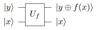
The quantum oracle \(U_f\) acts as

\(\ket{x}\ket{y} \xrightarrow{U_f} \ket{x}\ket{y \oplus f(x)}\)

For now, we will demonstrate a simple example of a quantum oracle. Consider \(f(x) = x\).

1.1 IBM Quantum Composer

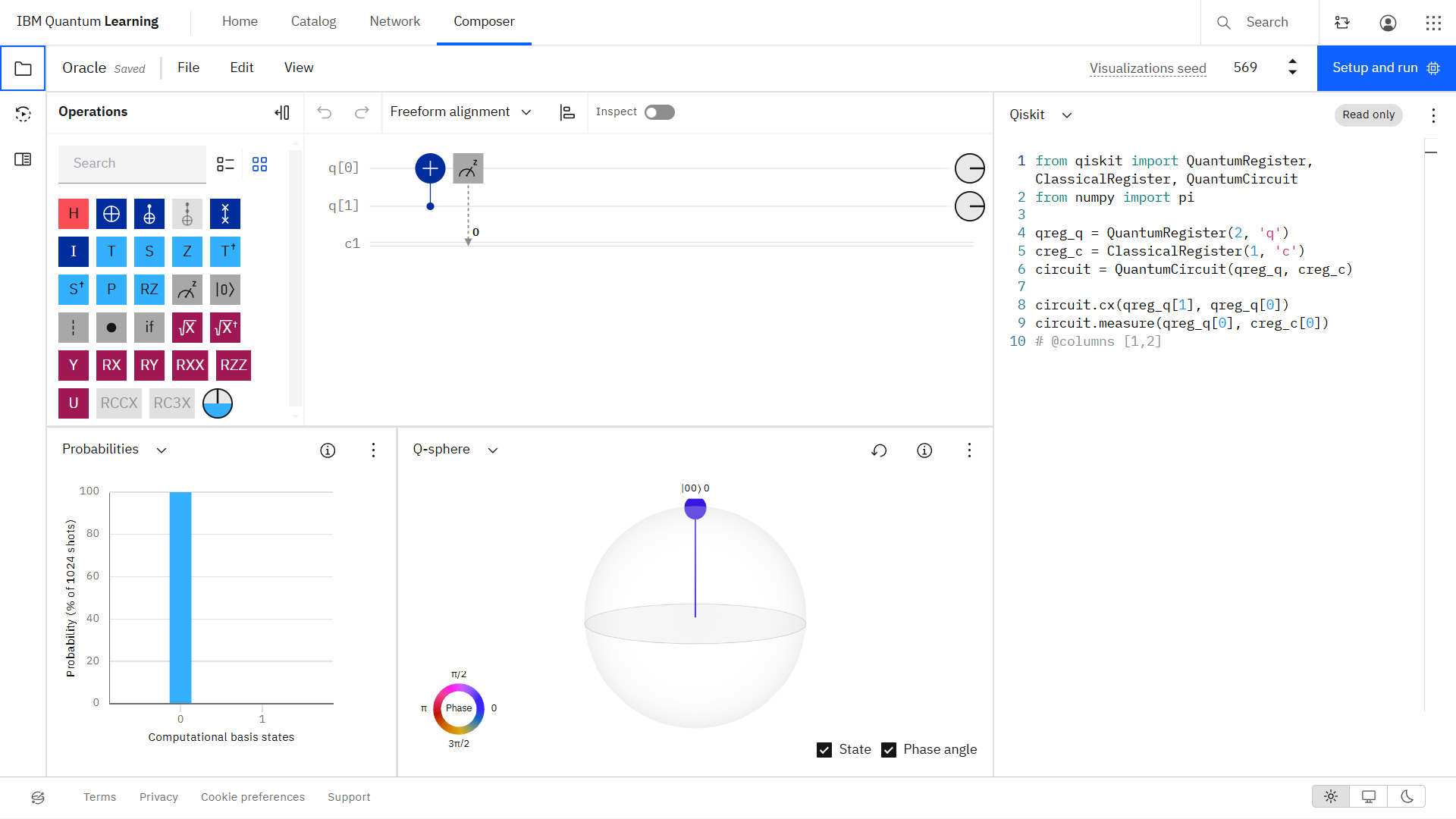
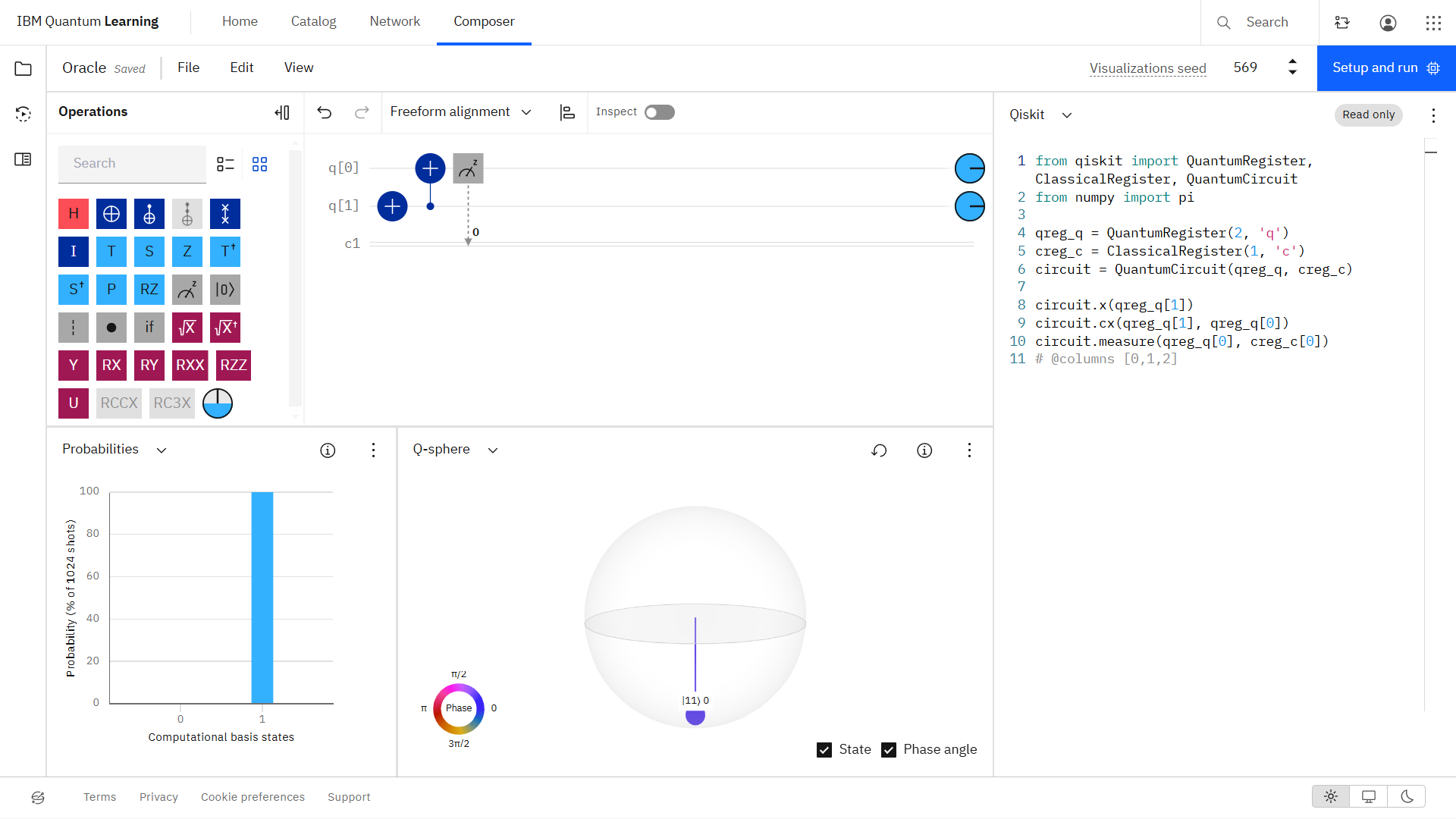
Let the first qubit be the input qubit \(x\) and the second qubit be the answer or target qubit \(y\). The result of \(f(x)\) is dependent on the input qubit, \(x\).

Setting \(y = \ket{0}\), we can find \(f(x)\) for \(x = \ket{0}, \ket{1}\).

\(\underline{x = \ket{0}, y = \ket{0}}\)   \(\left(\ket{0}\ket{0 \oplus 0}\right)\)

\(\underline{x = \ket{1}, y = \ket{0}}\)   \(\left(\ket{1}\ket{0 \oplus 1}\right)\)

1.2 Qiskit Implementation

from qiskit import QuantumCircuit

# Create a quantum circuit with 2 qubits and 1 classical bits
qc = QuantumCircuit(2, 1)

# Step 1: Start with |0> state for the first qubit (target qubit |y>)
# The qubits are initialized to |0> by default in Qiskit

# Step 2: Initialize the second qubit (|x>) to either |0> or |1>
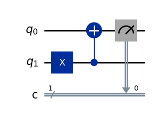
qc.x(1)  # Apply X gate to initialize |x> to |1> (remove this line for |x> = |0>)

# Step 3: Apply a CNOT gate with the second qubit as control and first qubit as target
qc.cx(1, 0)  # CNOT gate: |y> → |y ⊕ x|

# Step 4: Measure each qubit
qc.measure(0, 0)  # Measure the target qubit (|y ⊕ x|) into the first classical bit

# Visualize the circuit
qc.draw(output='mpl')

2. Phase Oracles

Previously, \(\ket{y} \rightarrow \ket{y \oplus x}\). Phase oracles, however, allow one to query a quantum oracle without changing the answer or target qubit, \(\ket{y}\).

To do this, we set \(\ket{y} = \ket{-}\). However, this change causes the input qubit, \(\ket{x}\), to change its phase, \(\ket{x} \xrightarrow{U_f} (-1)^{f(x)}\ket{x}\).

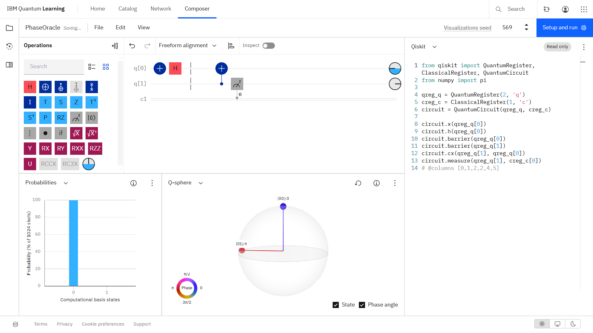
2.1 IBM Quantum Composer

Let the first qubit be the input qubit \(x\) and the second qubit be the answer or target qubit \(y\). First, we initialize \(\ket{y} = \ket{-}\), shown before the barriers below. Then we apply the oracle. This time, we measure the input qubit \(x\) because the answer or target qubit \(\ket{y}\) is unchanged.

\(\underline{x = \ket{0}, y = \ket{-}}\)   \(\left(\ket{0}\ket{- \oplus 0}\right)\)

\(\underline{x = \ket{1}, y = \ket{-}}\)   \(\left(\ket{1}\ket{- \oplus 1}\right)\)

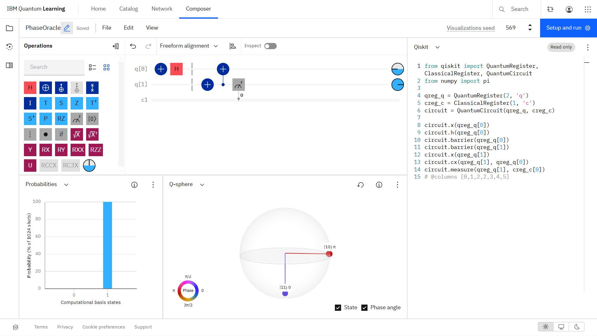
Notice the phase change compared to the previous quantum oracle implementation. This change is important for quantum algorithms.

2.2 Qiskit Implementation

# Create a quantum circuit with 2 qubits and 1 classical bits
qc = QuantumCircuit(2, 1)

# Step 1: Start with |-> state for the first qubit (target qubit |y>)
# The qubits are initialized to |0> by default in Qiskit
qc.x(0)
qc.h(0)

# Add barriers (to match composer construction)
qc.barrier(0)
qc.id(1)
qc.id(1)
qc.barrier(1)

# Step 2: Initialize the second qubit (|x>) to either |0> or |1>
qc.x(1)  # Apply X gate to initialize |x> to |1> (remove this line for |x> = |0>)

# Step 3: Apply a CNOT gate with the second qubit as control and first qubit as target
qc.cx(1, 0)  # CNOT gate: |y> → |y ⊕ x|

# Step 4: Measure each qubit
qc.measure(1, 0)  # Measure the input qubit (|x>) into the first classical bit

# Visualize the circuit
qc.draw(output='mpl')