Shor’s Algorithm

Shor’s Algorithm significantly enhances the efficiency of integer factorization, making it exponentially faster than classical methods.

1. Problem Statement

2. Shor’s Algorithm

3. Qiskit Implementation

4. Circuit Construction

5. Execution

6. Post Processing

1. Problem Statement

This problem involves factoring a given integer efficiently. Classical algorithms for integer factorization, such as trial division and the general number field sieve, are slow for large numbers. Shor’s Algorithm leverages quantum computing to solve this problem in polynomial time.

Given an integer N, the goal is to find its nontrivial factors (any factors other than 1 and N) using quantum techniques.

2. Shor’s Algorithm Steps

As an example, say we want to factor \(N = 15\).

Classical Preprocessing

Step 1. Choose a random integer \(a\):

• Pick \(a = 2\).

• Find the greatest common divisor: \(\gcd(a, N)\).

  • Since \(\gcd(2, 15)\) = 1 , we continue.

Greatest common divisor: The greatest common divisor of two integers is the largest number that divides both of them without leaving a remainder.

In the context of integer factorization, the GCD can immediately provide a nontrivial factor of 𝑁: - If \(\gcd(a, N) > 1\), then \(\gcd(a, N)\) is a divisor of N. This means we have already found a factor of N, and no further computation is needed. - If \(\gcd(a, N) = 1\), it means a and N are coprime. (i.e., they share no common factors other than 1). In this case, we must proceed with additional quantum techniques to factor N.

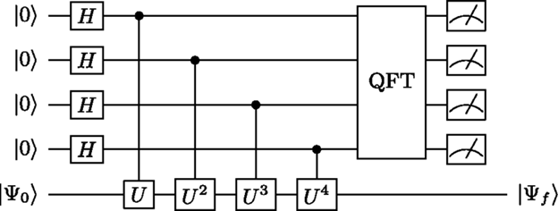
Quantum Period Finding - Quantum Phase Estimation (QPE)

Step 2. Find the period \(r\) of \(a\) mod N:

• The order \(r\) is the smallest integer such that: \(2^r =\mod{15}\).

• Quantum period-finding determines \(r\) = 4.

Classical Post-Processing

Step 3. Check if \(r\) is even:

• Since \(r = 4\) is even, we proceed.

Step 4. Compute potential factors of \(N\):

• Compute: \(a^{r/2}\) - 1 and \(a^{r/2}\) + 1.

• Compute gcd with \(N = 15\):

  \[p = \gcd(3, 15) = 3, \quad q = \gcd(5, 15) = 5\]

• This successfully factors \(15\) into \(3 \cdot 5\).

3. Qiskit Implemenation

3.1 Imports

%pip install numpy
%pip install qiskit
%pip install qiskit_ibm_runtime
%pip install qiskit_aer

import numpy as np
import math
from qiskit import QuantumCircuit
from qiskit.circuit.library import CUGate
from qiskit.transpiler.preset_passmanagers import generate_preset_pass_manager as gppm
from qiskit_ibm_runtime import QiskitRuntimeService, SamplerV2 as Sampler
from qiskit.visualization import plot_distribution
from qiskit_aer import AerSimulator

3.2 Quantum Phase Estimation

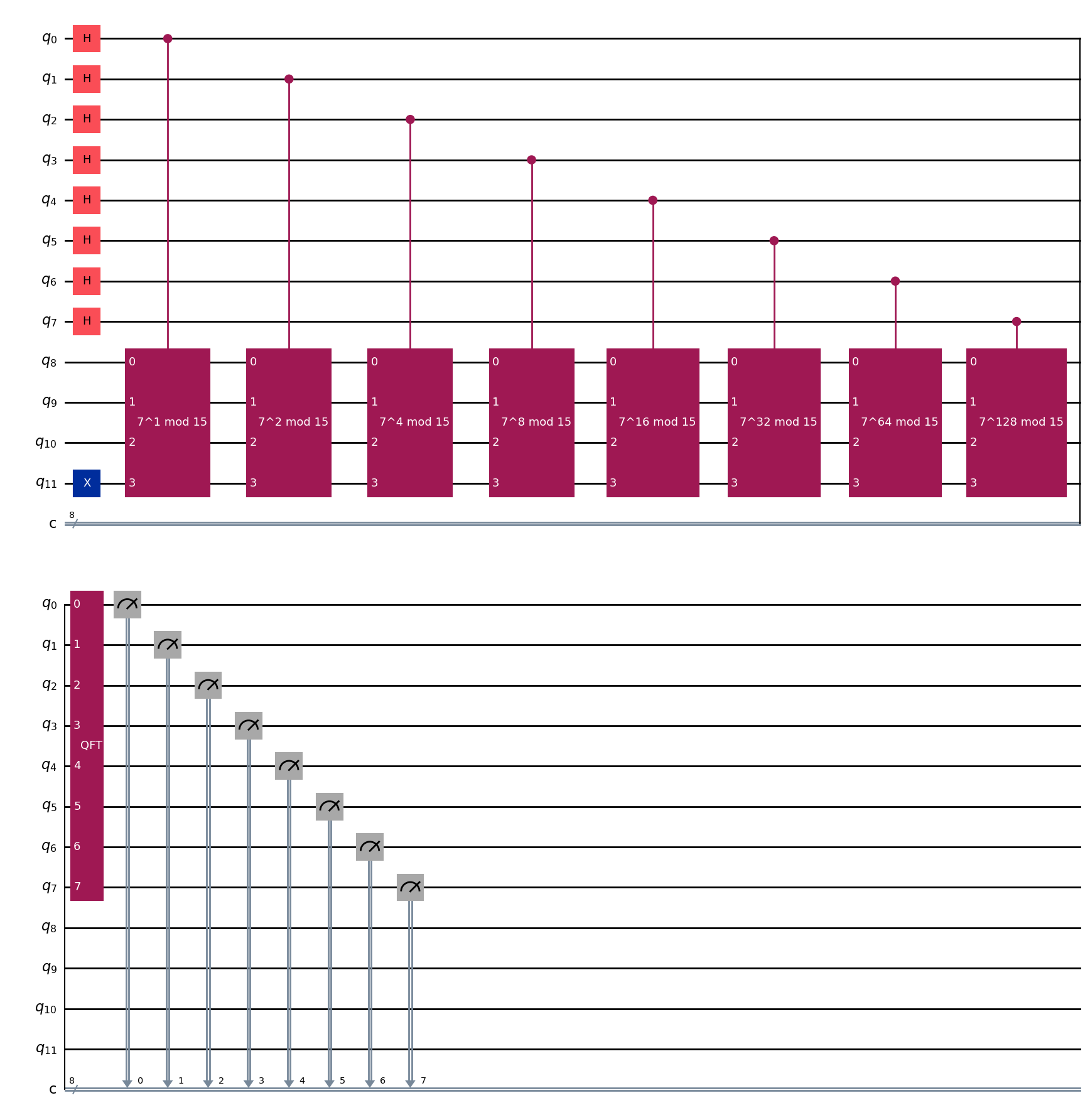
def c_amod15(a,power):
    U = QuantumCircuit(4)
    for _ in range(power):
        U.swap(2, 3)
        U.swap(1, 2)
        U.swap(0, 1)
        for q in range(4):
            U.x(q)
    U = U.to_gate()
    U.name = "%i^%i mod 15" %(a,power)
    c_U = U.control()
    return c_U

3.3 Quantum Fourier Transform

Finding \(r\) in polynomial time.

def qft(n):
    #Initialize quantum circuit
    qc = QuantumCircuit(n)
    for qubit in range(n//2):
        qc.swap(qubit, n-qubit-1)
    for j in range(n):
        for m in range(j):
            angle = -(np.pi/float(2**(j-m)))
            cu1_gate = CUGate(0,0,0,angle)
            qc.append(cu1_gate, [m, j])
        qc.h(j)
    qc.name = "QFT"
    return qc

4. Circuit Construction

n_count = 8
a = 7

qc = QuantumCircuit(n_count + 4, n_count)

for q in range(n_count):
    qc.h(q)

qc.x(3+n_count)

for q in range(n_count):
    qc.append(c_amod15(a,2**q), [q]+[i+n_count for i in range(4)])

qc.append(qft(n_count), range(n_count))
qc.measure(range(n_count), range(n_count))
qc.draw('mpl')

5. Execution

service = QiskitRuntimeService()
backend = AerSimulator()
pm = gppm(backend=backend, optimization_level = 1)
isa_circuit = pm.run(qc)
sampler = Sampler(backend)
job = sampler.run([isa_circuit], shots = 4096)

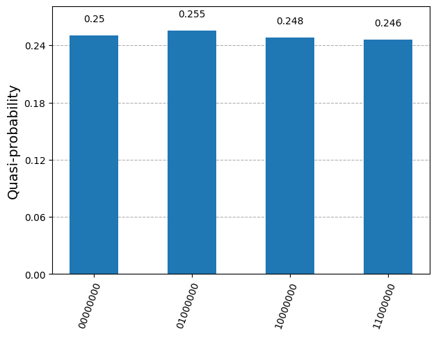
6. Post Processing

nums = job.result()[0].data.c.get_counts()
new = {
    '00000000':0,
    '01000000':0,
    '10000000':0,
    '11000000':0
}

denoms = set()
for key, value in nums.items():
    if(key[:2]=='00'):
        new['00000000'] += value
    elif(key[:2]=='01'):
        new['01000000'] += value
    elif(key[:2]=='10'):
        new['10000000'] += value
    elif(key[:2]=='11'):
        new['11000000'] += value

for key in new:
    gcd = math.gcd(int(key, 2), 2**n_count)
    denom = (2**n_count)//gcd
    if (denom%2==0 and (a**denom)%15 != 14):
        denoms.add((2**n_count)//gcd)

r = max(denoms)
p = (math.gcd(a**(r//2)-1, 15))
q = (math.gcd(a**(r//2)+1, 15))
print("The factors of 15 are " + str(p) + " and " + str(q) + ".")
plot_distribution(new)

The factors of 15 are 3 and 5.