Simon’s Algorithm
Simon’s algorithm is the first quantum algorithm to offer an exponential speedup over the best-known classical algorithm for Simon’s problem.
1. Problem Statement
Simon’s problem involves finding a secret \(n\)-bit string, \(s\), by querying an oracle that maps two distinct inputs to one unique output (a two-to-one function).
The oracle takes an \(n\)-bit string \(x = x_{n-1}\ldots x_1x_0\) as input and outputs an \(n\)-bit string \(f(x)=f_{n-1}\ldots f_1f_0\). The oracle promises that:
where \(y = x \oplus s\) and \(\oplus\) denotes a bitwise \(\text{XOR}\).
In other words, for every output value \(f(x)\), there exists exactly two distinct inputs \(x\) and \(y\) such that their \(\text{XOR}\) difference is the unknown string \(s\) (\(x \oplus y = s\)).
Our goal is to determine the unknown string \(s\) by querying the oracle.
1.1 Example
Consider the following simple example with \(n = 3\) and the secret string \(s = 110\).
\(x\) |
\(f(x\oplus s)\) |
|---|---|
000 |
101 |
001 |
010 |
010 |
011 |
011 |
100 |
100 |
011 |
101 |
100 |
110 |
101 |
111 |
010 |
Notice that inputs \(x = 000\) and \(x = 110\) will produce the same output \(f(x\oplus s) = 101\). This produces a collision, i.e. two inputs map to the same output.
The same relationship exists for \(x = 001 = 111\), \(x = 010 = 100\), and \(x = 011 = 101\).
1.2 Classical Solution
If we find a collision, we can find the hidden string \(s\) by taking the \(\text{XOR}\) of the two inputs:
One classical approach is the brute-force method, where you try each input one-by-one to find a collision. In the worst case, you could try half the inputs \((2^{n-1})\) before finding a collision.
For the best randomized classical algorithm, the number of queries is \(2^{\frac{n}{2}}\), which is still exponential.
2. Quantum Solution
To find the hidden string \(s\), Simon’s algorithm is required to run at least \(n\) times to retrieve different measurements, \(\ket{z}\), such that the dot product of \(s\) and \(z\) is \(0\):
For Simon’s algorithm, we need \(n\) input qubits and \(n\) answer qubits. In Deutsch’s and Bernstein’s algorithm, the answer qubits begin in the \(\ket{-}\) state. Here, we will begin all qubits in the \(\ket{0}\) state. In this example, the secret string \(s = 110\).

2.1 IBM Quantum Composer
IBM Quantum Composer: https://quantum.ibm.com/composer/
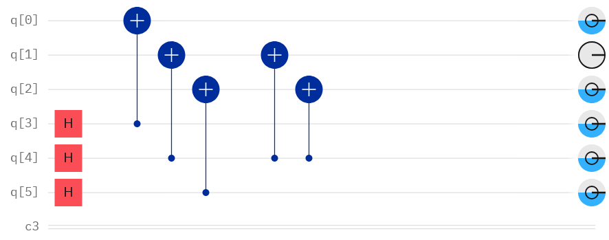
2.1.1 Preprocessing
We apply Hadamards to all input qubits. Note that the visualization of the Q-sphere does not work for \(5+\) qubits.

2.1.2 Oracle
Then we apply the oracle such that: \(\ket{x}\ket{0}\rightarrow\ket{x}\ket{x\oplus s}\).
First, we want to copy the inputs to their corresponding output register \(\left(\ket{x}\ket{0}\rightarrow\ket{x}\ket{x}\right)\). We do this by applying a CNOT with the input qubit as the control and the output qubit as the target.

Now, there are many ways to implement a two-to-one function. In this approach, we split the inputs into two groups based on the index of a chosen flag bit. For all inputs \(x\), if the bit at that index is \(1\), we \(\text{XOR}\) the input string with \(s\). This causes the following change in the oracle, \(\ket{x}\ket{x}\rightarrow\ket{x}\ket{x\oplus s}\) if the chosen bit is 1.
Since we want \(s\) to map to the zero string, we identify the index of the first bit in \(s\) that is a \(1\) to be the flag. In this case (\(s = 1\underline{1}0\)), the index of the chosen flag bit would be \(2\).
\(x\) |
\(f(x\oplus s)\) |
|---|---|
000 |
000 |
001 |
001 |
010 |
011 |
011 |
100 |
100 |
011 |
101 |
100 |
110 |
101 |
111 |
010 |
2.1.3 Postprocessing
Finally, apply Hadamards to all input qubits again and measure.

2.2 Classical Postprocessing
We will use the results in the probability distribution to classically find \(s\). The results must satisfy:
Therefore, we can construct a system of equations to solve for \(s\).
From the second equation, we can see \(s_0 = 0\).
From the last \(2\) equations, we can see \(s_2 = s_1 = 0\) \((s = 000)\) or \(s_2 = s_1 = 1\) \((s = 110)\). The non-trivial solution gives us \(s = 110\), which is our hidden string.
Computationally, we can solve this method with Gaussian Elimination with a runtime of \(O(n^3)\).
3. Qiskit Implementation
For our Qiskit implementation, we set the secret string \(s = 11010\).
Imports
[ ]:
%pip install qiskit
%pip install qiskit_ibm_runtime
%pip install qiskit_aer
%pip install numpy
%pip install scipy
[1]:
import qiskit
print(qiskit.version.get_version_info())
1.2.4
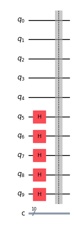
3.1 Circuit Construction
[2]:
from qiskit import QuantumCircuit

# Preprocessing
# Select a secret bit string
s = '11010'

# Number of qubits to represent s
num_qubits = num_bits = len(s)

# Create a circuit with num_qubits + ancilla, and num_bits
qc = QuantumCircuit(2 * num_qubits, 2 * num_bits)

# Apply Hadamards to all input qubits
qc.h(range(num_qubits, 2 * num_qubits))

qc.barrier()

qc.draw(output="mpl", scale=0.6)
[2]:
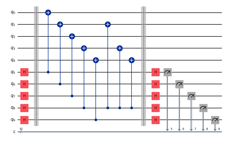
[3]:
# Oracle
# Reverse s to fit Qiskit's qubit ordering (bottom up 11010 -> top down 01011)
reverse_s = s[::-1]

flag_bit = reverse_s.find("1")

# |x>|0> -> |x>|x>
# Copy input to output
for q in range(num_qubits):
    qc.cx(q + num_qubits, q)

# |x> -> |x ⊕ s>
# If there is a found chosen flag bit, apply CNOT with flag as control and
if flag_bit != -1:
    for q in range(num_qubits):
        if reverse_s[q] == '1':
            qc.cx(2 * num_qubits - (flag_bit + 1), q)

qc.barrier()

qc.draw(output="mpl", scale=0.6)
[3]:

[4]:
# Post processing and measurement
# Apply Hadamards to all input qubits
qc.h(range(num_qubits, 2 * num_qubits))

# Measure input qubits
for q in range(num_qubits, 2 * num_qubits):
    qc.measure(q, q)

qc.draw(output="mpl", scale=0.6)
[4]:
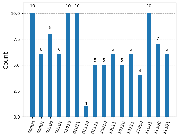
3.2 Running on a Simulator
First, we initialize a StatevectorSampler primitive that classically simulates the execution of quantum circuits. Then, we run the primitive with \(n + 100\) shots and retrieve its results.
[5]:
# Running on Simulator
from qiskit.primitives import StatevectorSampler
from qiskit.visualization import plot_histogram

sampler = StatevectorSampler()

sim_qc = qc

# Run using sampler n + 2 times to ensure we have at least n measurements
result = sampler.run([sim_qc], shots=num_qubits + 100).result()

# Get counts for the classical register "c" (Note that the unmeasured qubits remain in the final result)
counts = result[0].data.c.get_counts()
print(f"The counts are: {counts}")

# Remove unmeasured qubits from final result
final_counts = {}
for key, value in counts.items():
    measured = key[:num_qubits]
    final_counts[measured] = value

plot_histogram(final_counts)
The counts are: {'0111100000': 5, '1001000000': 5, '1110100000': 6, '1100000000': 4, '0010000000': 8, '0000000000': 10, '0000100000': 6, '1011000000': 5, '1110000000': 7, '1100100000': 10, '1011100000': 6, '0101100000': 10, '0101000000': 10, '0010100000': 6, '1001100000': 6, '0111000000': 1}
[5]:
3.3 Classical Postprocessing
We prepare the measurements as a matrix of integers, utilize Sympy’s RREF function to compute the reduced row echelon form of the matrix, and identify the null space of the matrix (\(A \cdot x = 0\)), which corresponds to the solution of the system of linear equations. Note that sometimes the choice of bitstrings for the systems of equations may not be linearly independent and result in an incorrect solution.
[6]:
import numpy as np
from sympy import Matrix

# Sort by highest frequency and take only the first n measurements
final_counts = dict(sorted(final_counts.items(), key=lambda item: item[1], reverse=True))
first_n_measured = dict(list(final_counts.items())[:num_qubits])
print("First n measured:", first_n_measured)

# Convert measurements to matrix of integers
matrix = np.array([list(bitstring) for bitstring, count in first_n_measured.items()]).astype(int)
print("\nMatrix:")
for i in range(len(matrix)):
    print(matrix[i])

# Transpose the matrix and append identity matrix
matrix = Matrix(matrix).T
augmented_matrix = Matrix(np.hstack([matrix, np.eye(matrix.shape[0], dtype=int)]))

# Perform Gauss-Jordan elimination to reduce matrix to reduced row echelon form (RREF) mod 2
reduced_row = augmented_matrix.rref(iszerofunc=lambda x: x % 2 == 0)
print("\nRow reduced:\n", reduced_row)

# Convert from Sympy Matrix object to np array mod 2
final_result = np.array(reduced_row[0])
final_result = np.mod(final_result, 2)
print("\nFinal result:")
for i in range(len(final_result)):
    print(final_result[i])

# Retrieve solution in the last row of reduced matrix, if the last row of the rref is all 0
if all(value == 0 for value in final_result[-1, :matrix.shape[1]]):
    result = "".join(str(c) for c in final_result[-1, matrix.shape[1]:])
else:
    result = "0" * matrix.shape[0]

assert(result == s)

print("\nResult:", result)
print("Hidden bitstring s:", s)
First n measured: {'00000': 10, '11001': 10, '01011': 10, '01010': 10, '00100': 8}

Matrix:
[0 0 0 0 0]
[1 1 0 0 1]
[0 1 0 1 1]
[0 1 0 1 0]
[0 0 1 0 0]

Row reduced:
 (Matrix([
[0, 1, 0, 0, 0, 0,  1, 0, -1,  0],
[0, 0, 1, 0, 0, 0, -1, 0,  1,  1],
[0, 0, 0, 1, 0, 0,  1, 0,  0, -1],
[0, 0, 0, 0, 1, 0,  0, 1,  0,  0],
[0, 0, 0, 0, 0, 1, -1, 0,  1,  0]]), (1, 2, 3, 4, 5))

Final result:
[0 1 0 0 0 0 1 0 1 0]
[0 0 1 0 0 0 1 0 1 1]
[0 0 0 1 0 0 1 0 0 1]
[0 0 0 0 1 0 0 1 0 0]
[0 0 0 0 0 1 1 0 1 0]

Result: 11010
Hidden bitstring s: 11010
4. Firsthand Experience with ibm_rensselaer
As usual, we initialize the QiskitRuntimeService to interact with IBM Quantum resources.
If you have not already, use the following snippet to log in and save your IBM Quantum account credentials for future use. Replace the token with your own API token available when you log in at https://quantum.ibm.com/.
[7]:
from qiskit_ibm_runtime import QiskitRuntimeService

# QiskitRuntimeService.save_account(
#     channel="ibm_quantum",
#     token="token",
#     set_as_default=True,
#     # Use 'overwrite=True' if you're updating your token.
#     overwrite=True,
# )
[8]:
service = QiskitRuntimeService()

# Should be "ibm_rensselaer". If not and you have access to the computer, comment this out and set the backend manually.
# backend = service.least_busy(operational=True, simulator=False)
# print(backend.name)

backend = service.backend("ibm_rensselaer")
print(backend.name)
ibm_rensselaer
ibm_rensselaer.ibm_rensselaer. This can take a couple of minutes or more, depending on the job queue.[9]:
from qiskit.transpiler.preset_passmanagers import generate_preset_pass_manager

pm = generate_preset_pass_manager(target=backend.target, optimization_level=1)

isa_circuit = pm.run(qc)
# isa_circuit.draw(output='mpl',scale=0.5)
To account for noise, we run the circuit for \(1000\) shots and then select the first \(n\) measurements with the highest counts.
[10]:
from qiskit_ibm_runtime import SamplerV2 as Sampler

sampler = Sampler(mode=backend)

# Use 1000 shots
job = sampler.run([isa_circuit], shots=1000)
job_result = job.result()
counts = job_result[0].data.c.get_counts()

print(f"The counts are: {counts}")

# Remove unmeasured qubits from final result
final_counts = {}
for key, value in counts.items():
    measured = key[:num_qubits]
    final_counts[measured] = value

plot_histogram(final_counts)
The counts are: {'1101000000': 33, '0001000000': 33, '1011100000': 60, '0111100000': 55, '0101000000': 48, '1001100000': 44, '1001000000': 56, '0101100000': 51, '1000100000': 15, '1110000000': 33, '1111000000': 29, '0100000000': 13, '1111100000': 38, '1100100000': 23, '0010100000': 27, '1101100000': 37, '0000100000': 27, '0100100000': 16, '0011100000': 25, '0010000000': 38, '0111000000': 41, '1010000000': 17, '0001100000': 33, '1011000000': 54, '1000000000': 18, '1010100000': 19, '0110100000': 14, '0110000000': 15, '0011000000': 28, '0000000000': 18, '1100000000': 20, '1110100000': 22}
[10]:

After running the circuit, we classically postprocess the results. Before taking the first \(n\) measurements, the final counts are sorted in reverse order. Note that noise in the quantum system may produce incorrect bitstring outputs and, as a result, cause indeterminate solutions.
[11]:
import numpy as np
from sympy import Matrix

# Sort by highest frequency and take only the first n measurements
final_counts = dict(sorted(final_counts.items(), key=lambda item: item[1], reverse=True))
first_n_measured = dict(list(final_counts.items())[:num_qubits])
print("First n measured:", first_n_measured)

# Convert measurements to matrix of integers
matrix = np.array([list(bitstring) for bitstring, count in first_n_measured.items()]).astype(int)
print("\nMatrix:")
for i in range(len(matrix)):
    print(matrix[i])

# Transpose the matrix and append identity matrix
matrix = Matrix(matrix).T
augmented_matrix = Matrix(np.hstack([matrix, np.eye(matrix.shape[0], dtype=int)]))

# Perform Gauss-Jordan elimination to reduce matrix to reduced row echelon form (RREF) mod 2
reduced_row = augmented_matrix.rref(iszerofunc=lambda x: x % 2 == 0)
print("\nRow reduced:\n", reduced_row)

# Convert from Sympy Matrix object to np array mod 2
final_result = np.array(reduced_row[0])
final_result = np.mod(final_result, 2)
print("\nFinal result:")
for i in range(len(final_result)):
    print(final_result[i])

# Retrieve solution in the last row of reduced matrix, if the last row of the rref is all 0
if all(value == 0 for value in final_result[-1, :matrix.shape[1]]):
    result = "".join(str(c) for c in final_result[-1, matrix.shape[1]:])
else:
    result = "0" * matrix.shape[0]

assert(result == s)

print("\nResult:", result)
print("Hidden bitstring s:", s)
First n measured: {'10111': 60, '10010': 56, '01111': 55, '10110': 54, '01011': 51}

Matrix:
[1 0 1 1 1]
[1 0 0 1 0]
[0 1 1 1 1]
[1 0 1 1 0]
[0 1 0 1 1]

Row reduced:
 (Matrix([
[1, 0, 0, 0,  0, 0, -1,  0,  0,  1],
[0, 1, 0, 0,  1, 0,  0, -1,  1,  0],
[0, 0, 1, 0,  1, 0,  1,  0,  0,  0],
[0, 0, 0, 1, -1, 0,  0,  1,  0, -1],
[0, 0, 0, 0,  0, 1,  1,  0, -1,  0]]), (0, 1, 2, 3, 5))

Final result:
[1 0 0 0 0 0 1 0 0 1]
[0 1 0 0 1 0 0 1 1 0]
[0 0 1 0 1 0 1 0 0 0]
[0 0 0 1 1 0 0 1 0 1]
[0 0 0 0 0 1 1 0 1 0]

Result: 11010
Hidden bitstring s: 11010