Markov Decision Process (MDP) Modelings

We propose three different ways to model the quantum circuit design (QCD) task within a Markov Decision Process (MDP) framework:

1. Matrix Representation

2. Reverse Matrix Representation

3. Tensor Network (TN) Representation

In each MDP modeling, we define the following three key components:

1. State Space: The set of all possible states that can arise during circuit construction, where each state represent a partial circuit

2. Action Set:

   • The set of all possible gates that can be applied at any point, e.g., \(H\), \(T\), or \(\text{CNOT}\) on specific qubit(s).

   • Executing an action transforms one state into another by adding the chosen gate to the circuit.

3. Reward Function:

   • A measure of how close the resulting state is to the target operation.

We will use the Bell-state circuit in Fig. 1 as a running example to illustrate these approaches.

Matrix Representation: A Step-by-Step Overview

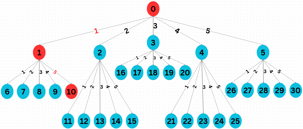
Fig. 2 State tree in matrix representation for searching the circuit in Fig. 1.

A Gentle Single-Qubit Example

Before we explore the 4×4 matrix representation for the two-qubit Bell state, let’s build some intuition with a simpler single-qubit scenario.

1. Initial Matrix: For a single qubit, the identity matrix is \(I_2 = \begin{pmatrix}1 & 0 \\ 0 & 1\end{pmatrix}\). Think of this as your “starting state,” which does nothing to the qubit.

2. Apply a Gate: For instance, applying the Hadamard gate \(H\) (an action \(a = H\)) transforms the state via matrix multiplication: \(H \cdot I_2 = H\).

3. Result: Once you apply a gate, the new matrix represents the updated transformation on your qubit.

In this way, each action (i.e., choosing a gate) updates the overall transformation by multiplying the current matrix with the gate’s matrix. Now, let’s extend this idea to two-qubit matrices of size 4×4.

Matrix Representation (Two-Qubit)

• Actions \(\mathcal{A}\) = { \(H_0, H_1, T_0, T_1, \text{CNOT}_{01}\) }. These five gates act on either qubit \(q_0\) or \(q_1\). An action \(a \in \mathcal{A}\) is thus a \(4 \times 4\) matrix.

• State Space \(\mathcal{S}\): The initial state is \(U_0 = I_{4}\), the \(4 \times 4\) identity matrix. The terminal state is \(U\), given in (2). Let \(S\) be the current state (a node in Fig. 2), and \(A \in \mathcal{A}\) be the chosen action. Then the resulting child state \(S'\) is:

  (3)\[S' = A \cdot S\]

  In other words, we transform the existing matrix \(S\) by multiplying on the left by the gate matrix \(A\).

• Tree Structure: As shown in Fig. 2, from the initial state \(S_0 = I_4\), we have 5 possible actions, leading to { \(S_1, S_2, S_3, S_4, S_5\) }. Another step of 5 actions from any of those states yields 25 more states, and so on. Altogether, \(\mathcal{S}\) contains 31 states in this example.

• Reward Function \(\mathcal{R}\): At state \(S_1\), if the agent picks \(\text{CNOT}_{01}\), then \(R(s = S_1, a = \text{CNOT}_{01}) = 100\); otherwise \(R(s,a) = 0\).

Example for Fig. 1

Suppose the initial state is \(S_0 = I_4\), and we follow the optimal path \(S_0 \rightarrow S_1 \rightarrow S_{10}\):

1. State after first action \(a = H_0\):

   (4)\[\begin{split}S_1 = (H_0 \otimes I) S_0 = \frac{1}{\sqrt{2}} \begin{pmatrix} 1 & 0 & 1 & 0 \\ 0 & 1 & 0 & 1 \\ 1 & 0 & -1 & 0 \\ 0 & 1 & 0 & -1 \end{pmatrix}.\end{split}\]

2. State after second action \(a = \text{CNOT}_{01}\):

   (5)\[\begin{split}S_{10} &= \text{CNOT}_{01} \cdot S_1 \\ &= \frac{1}{\sqrt{2}} \begin{pmatrix} 1 & 0 & 0 & 0 \\ 0 & 1 & 0 & 0 \\ 0 & 0 & 0 & 1 \\ 0 & 0 & 1 & 0 \end{pmatrix} \begin{pmatrix} 1 & 0 & 1 & 0 \\ 0 & 1 & 0 & 1 \\ 1 & 0 & -1 & 0 \\ 0 & 1 & 0 & -1 \end{pmatrix} = U,\end{split}\]

   This final matrix \(U\) corresponds to the target circuit in (2).

Advantages and Disadvantages

• Advantage: Because different gate sequences can produce the same overall \(4 \times 4\) matrix, this representation can merge multiple paths into a single state, reducing the search space.

• Disadvantage: The RL agent must be re-trained for each target matrix, even if many circuits share common intermediate sub-matrices.

Reverse Matrix Representation

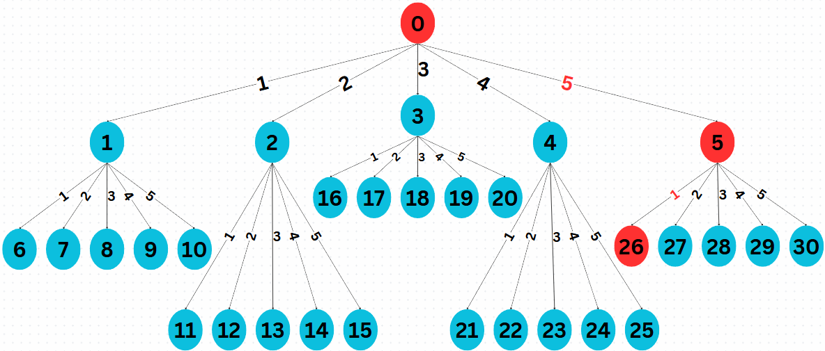
Fig. 3 State tree in reverse matrix representation for searching the circuit in Fig. 1.

• Actions \(\mathcal{A}^{-1}\) = { \(H_0^{-1}, H_1^{-1}, T_0^{-1}, T_1^{-1}, \text{CNOT}_{01}^{-1}\) }. Each inverse gate is again a \(4 \times 4\) matrix.

• State Space \(\mathcal{S}^{-1}\): The initial state is now \(S_0^{-1} = U\) (the target matrix), and the terminal state is \(I_4\). Let \(S^{-1}\) be the current node in Fig. 3, and \(A^{-1} \in \mathcal{A}^{-1}\) be the chosen inverse gate. Then:

  (6)\[S'^{-1} = A^{-1} \cdot S^{-1}\]

  Similarly, this forms a tree with 31 states, just in the reverse direction.

• Reward Function \(\mathcal{R}\): If at state \(S_5^{-1}\) the agent picks \(H_0^{-1}\), we get \(R(s = S_5^{-1}, a = H_0^{-1})= 100\); otherwise 0.

Example for Fig. 1

Given \(S_0^{-1} = U\), we look at the optimal path \(S_0^{-1} \rightarrow S_5^{-1} \rightarrow S_{26}^{-1}\):

1. Applying \(\text{CNOT}_{01}^{-1}\):

   (7)\[\begin{split}S_5^{-1} = \text{CNOT}_{01}^{-1} \cdot S_0^{-1} = \begin{pmatrix} 1 & 0 & 0 & 0 \\ 0 & 1 & 0 & 0 \\ 0 & 0 & 0 & 1 \\ 0 & 0 & 1 & 0 \end{pmatrix} \frac{1}{\sqrt{2}} \begin{pmatrix} 1 & 0 & 1 & 0 \\ 0 & 1 & 0 & 1 \\ 0 & 1 & 0 & -1 \\ 1 & 0 & -1 & 0 \end{pmatrix} = \frac{1}{\sqrt{2}} \begin{pmatrix} 1 & 0 & 1 & 0 \\ 0 & 1 & 0 & 1 \\ 1 & 0 & -1 & 0 \\ 0 & 1 & 0 & -1 \end{pmatrix}.\end{split}\]

2. Applying \(H_0^{-1}\):

   (8)\[\begin{split}S_{26}^{-1} = (H_0^{-1} \otimes I) \cdot S_5^{-1} = \frac{1}{2} \begin{pmatrix} 1 & 0 & 1 & 0 \\ 0 & 1 & 0 & 1 \\ 1 & 0 & -1 & 0 \\ 0 & 1 & 0 & -1 \end{pmatrix} \begin{pmatrix} 1 & 0 & 1 & 0 \\ 0 & 1 & 0 & 1 \\ 1 & 0 & -1 & 0 \\ 0 & 1 & 0 & -1 \end{pmatrix} = I_4.\end{split}\]

Reversing the sequence of actions (and taking inverses) essentially shows you how to “unbuild” the target matrix \(U\) back to the identity.

Advantages

Different circuits share the same target, the identity matrix, which means they are likely to share common sub-matrices as they get close to the target. Therefore, RL agents can use prior experience from other circuits to avoid redundant training.

Tensor Network Representation

Fig. 4 TN representation of Fig. 1.

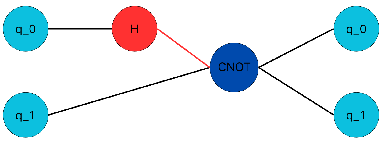
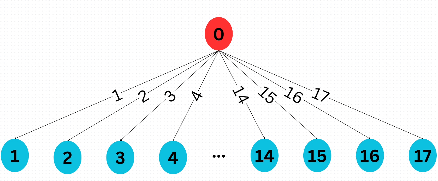
Fig. 5 State tree in TN representation for searching the circuit in Fig. 1.

The Tensor Network (TN) is another way to represent quantum circuits. Each gate becomes a tensor: single-qubit gates are 2-index tensors, two-qubit gates are 4-index tensors, etc. The network forms by connecting these tensors along shared indices.

For Fig. 1, consider the universal gate set \(G = \{ H_0, H_1, T_0, T_1, \text{CNOT}_{01} \}\). We allow up to two gates in one action for demonstration:

• Actions \(\mathcal{A}\) could be single gates or pairs of gates, e.g., \((H_0, \text{CNOT}_{01}), (\text{CNOT}_{01}, T_1), \ldots\) There are 17 distinct actions in total.

• State Space \(\mathcal{S}\): The initial state is \(S_0 = \ket{00}\), and the terminal state is the Bell state \(\ket{\Phi^+}\) in (1). The transition rule is analogous:

  (9)\[S' = A \cdot S\]

  where \(A\) acts on the current TN to produce a new one.

Example for Fig. 1

Starting with \(S_0 = \ket{00}\), we choose the combined action \((H_0, \text{CNOT}_{01})\):

(10)\[\begin{split}S_{14} &= \text{CNOT}_{01} \cdot (H \otimes I) \cdot S_0 \\ &= \text{CNOT}_{01} \cdot \Bigl(\tfrac{1}{\sqrt{2}}\bigl[\ket{00} + \ket{10}\bigr]\Bigr) \\ &= \tfrac{1}{\sqrt{2}}\bigl[\ket{00} + \ket{11}\bigr],\end{split}\]

which directly yields the Bell state.

Beginner’s Tip: In all three representations (Matrix, Reverse Matrix, and TN), you can think of state as “where you are” in the circuit-building process, and action as “which gate(s) to apply next.” The main difference is whether you are multiplying by the gate matrix or its inverse, or rewriting the system in a tensor form.

[Paper]

Wang, Z.; Feng, C.; Poon, C.; Huang, L.; Zhao, X.; Ma, Y.; Fu, T.; and Liu, X.-Y. 2025. Reinforcement learning for quantum circuit design: Using matrix representations. In arXiv, 2501.16509. https://arxiv.org/abs/2501.16509.