Algorithms
In this section, we explore two reinforcement learning (RL) methods for quantum circuit design: Q-learning (which uses a simple table to store Q-values) and Deep Q-Network (DQN) (which uses a neural network to approximate those values). We’ll discuss how each method updates its estimates of “how good” each state-action pair is, and how that helps our agent find optimal gate sequences.
Q-Learning
Q-learning is one of the simplest forms of RL. It learns a Q-table that tracks expected rewards (Q-values) for each possible state-action pair. When an agent takes an action, it observes a reward and updates its Q-table accordingly.
The update rule is:
where:
\(S_t\) and \(A_t\) are the current state and action.
\(S_{t+1}\) is the next state after taking the action.
\(R_{t+1}\) is the immediate reward for transitioning to the new state.
\(\alpha\) is the learning rate (how strongly we update the Q-value).
\(\gamma\) is the discount factor (how much we value future rewards).
Over many episodes of trial-and-error, Q-learning gradually refines its Q-table until it converges on an effective circuit-building strategy.
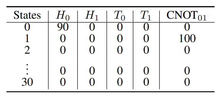
Fig. 6 Example Q-table for Bell state \(\ket{\Psi^+}\) after 500 iterations. At state 0, we take the action with the highest Q-value, \(H\). At state 1, we take the CNOT gate to construct \(\ket{\Psi^+}\).
Weakness of Q-Learning
A major drawback of Q-learning is scalability. In Q-learning, we store all Q-values in a table (the Q-table), where each entry corresponds to a state-action pair. As the state space and action space grow (e.g., more qubits, more gates), the size of this table can become prohibitively large. This makes classical Q-learning infeasible for many real-world quantum circuit design tasks, where the number of possible partial circuits explodes combinatorially.
To address this scalability issue, we need more compact ways to represent Q-values. This leads us to Deep Q-Networks (DQN) and other function approximators, which replace the Q-table with a neural network. Instead of explicitly storing one value per state-action pair, DQN learns a function that approximates these Q-values for any given state and action. This allows the algorithm to handle significantly larger or continuous state spaces.
DQN
Deep Q-Network (DQN) is a more advanced version of Q-learning that can handle large or continuous state spaces. Instead of storing Q-values in a table, we use a neural network to output estimates of Q-values for each action.
Key Components
Policy Network:
Parameterized by \(\theta\).
We typically have several fully connected layers (e.g., three layers, each with 128 neurons) taking the state as input and outputting Q-values for all possible actions.
Target Network:
Parameterized by \(\overline{\theta}\).
A separate, slowly updated network that helps stabilize training.
Periodically copied or softly updated from the policy network: \(\overline{\theta} \leftarrow (1-\alpha) \overline{\theta} + \alpha \theta\).
Replay Buffer:
Stores “experience tuples”: (state, action, reward, next_state).
We randomly sample from this buffer to reduce correlations between consecutive steps, making training more stable and efficient.
Training the Policy Network
We train the policy network to minimize the Mean Squared Error (MSE) between its predicted Q-values and the target Q-values. At each training step, we sample a mini-batch of experiences from the replay buffer and compute:
where:
\(Q(s, a \mid \theta)\) is the Q-value predicted by the policy network for the current state-action pair.
\(R\) is the reward for taking action \(a\) in state \(s\).
\(s'\) is the next state.
\(\max_{a'} Q(s', a' \mid \overline{\theta})\) is the estimated best future reward for next state \(s'\), as given by the target network.
This training loop typically runs in tandem with an exploration policy (e.g., \(\epsilon\)-greedy), so the network can keep discovering new gate sequences.
Training Process
Initialization:
Set up Q-table (for Q-learning) or neural networks (for DQN).
Define the environment (initial circuit state, target state, reward scheme).
Initialize replay buffer for DQN (if applicable).
Main RL Loop (for multiple episodes or iterations):
Reset the circuit to the initial state.
Select an action (gate choice) based on the current policy (exploration vs. exploitation).
Observe the new state and reward after applying the gate.
Update the Q-table or neural network (policy) using the formulas shown above.
If target state is reached or a max step limit is reached, end the episode.
Policy Improvement:
Over time, Q-values become more accurate, guiding the selection of actions that build the target circuit quickly and reliably.
In the upcoming sections, we will show how these methods can be applied to generate specific quantum circuits—like the Bell state, GHZ state, or multi-qubit gates, using the three representation methods.
Wang, Z.; Feng, C.; Poon, C.; Huang, L.; Zhao, X.; Ma, Y.; Fu, T.; and Liu, X.-Y. 2025. Reinforcement learning for quantum circuit design: Using matrix representations. In arXiv, 2501.16509. https://arxiv.org/abs/2501.16509.