Bloch Sphere
The Bloch sphere is a geometric representation used in quantum mechanics to visualize the state of a single qubit, which is the fundamental unit of quantum information. It represents qubit states as points on the surface of a unit sphere, where each point on the sphere corresponds to a specific quantum state. We will demonstrate these states using Qiskit.
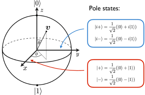
1. General Representation of a Qubit on the Bloch Sphere
A general single-qubit state \(\ket{\psi}\) can be written as:
1.1 Utilizing Qiskit - IBM Quantum Documentation
We use Qiskit’s built-in visualization function to help us plot the states on the Bloch Sphere.
qiskit.visualization.plot_bloch_vector(bloch, title=’’, ax=None, figsize=None, coord_type=’cartesian’, font_size=None)
We focus on the inputs to bloch and coord_type.
bloch (list[double]) – array of three elements where [<x>, <y>, <z>] (Cartesian) or [<r>, <theta>, <phi>] (spherical in radians)
coord_type (str) – a string that specifies coordinate type for bloch (Cartesian or spherical), default is Cartesian
More documentation for this function is available here: https://docs.quantum.ibm.com/api/qiskit/qiskit.visualization.plot_bloch_vector
Imports
[ ]:
%pip install qiskit
%pip install numpy
[1]:
from qiskit.visualization import plot_bloch_vector
import numpy as np
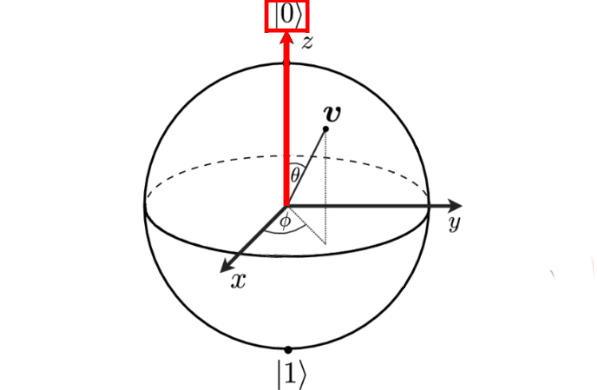
2. Computational Basis States (Z-Basis)
The computational basis states \(\ket{0}\) and \(\ket{1}\) are represented at the North and South poles of the Bloch Sphere, respectively.
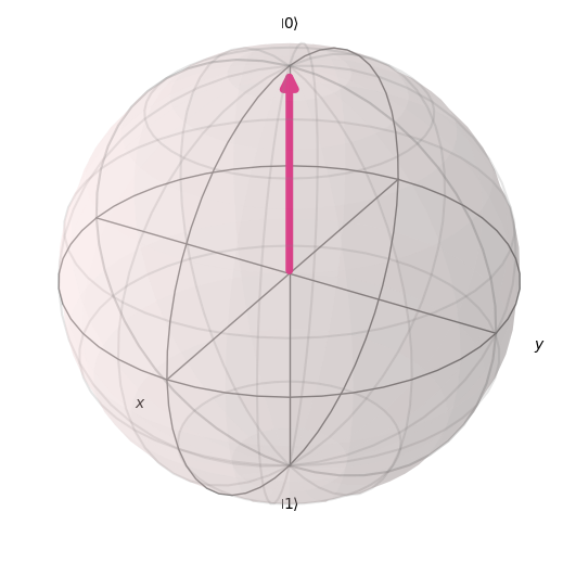
2.1 \(\ket{0}\)
Using Qiskit, we plot the state \(\ket{0}\) in Cartesian and polar coordinates.
[2]:
#cartesian coordinates
plot_bloch_vector([0, 0, 1], coord_type='cartesian')
[2]:

[3]:
#polar coordinates
plot_bloch_vector([1, 0, 0], coord_type='spherical')
[3]:
2.2 \(\ket{1}\)
Using Qiskit, we plot the state \(\ket{1}\) in Cartesian and polar coordinates.
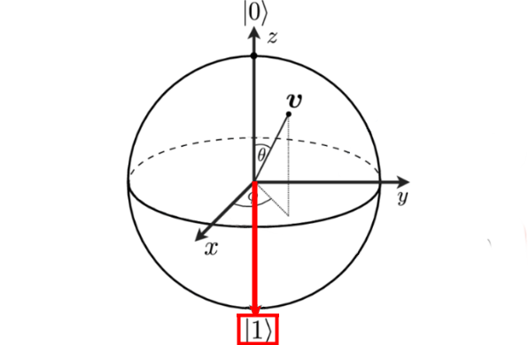
[4]:
#cartiesian coordinates
plot_bloch_vector([0, 0, -1], coord_type='cartesian')
[4]:

[5]:
#polar coordinates
plot_bloch_vector([1, np.pi, 0], coord_type='spherical')
[5]:

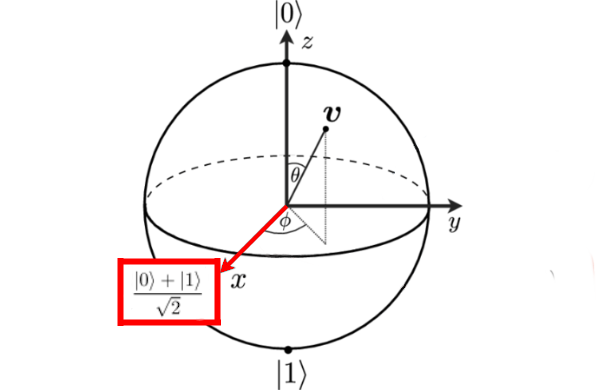
3. X-Basis States
\(\ket{+}\) and \(\ket{-}\) are located on the \(x\)-axis of the Bloch Sphere.
3.1 \(\ket{+}\)
The \(\ket{+}\) state lies on the positive \(x\)-axis, and is defined as:
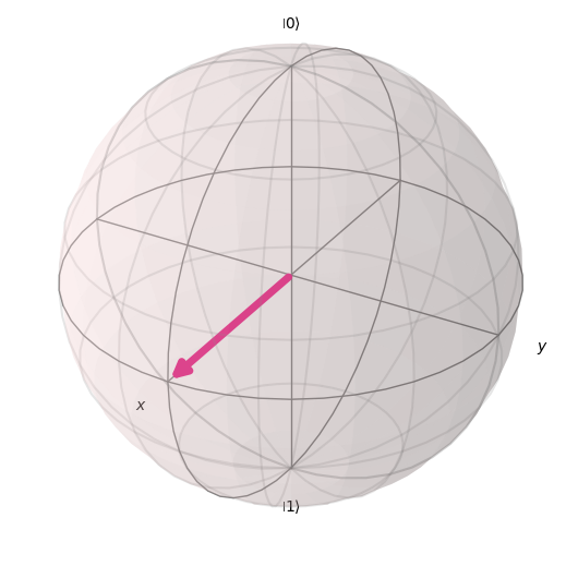
Using Qiskit, we plot the state \(\ket{+}\) in Cartesian and polar coordinates.
[6]:
#cartesian coordinates
plot_bloch_vector([1, 0, 0], coord_type='cartesian')
[6]:
[7]:
#polar coordinates
plot_bloch_vector([1, np.pi/2, 0], coord_type='spherical')
[7]:

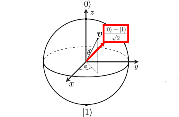
3.2 \(\ket{-}\)
The \(\ket{-}\) state lies on the negative \(x\)-axis, and is defined as:
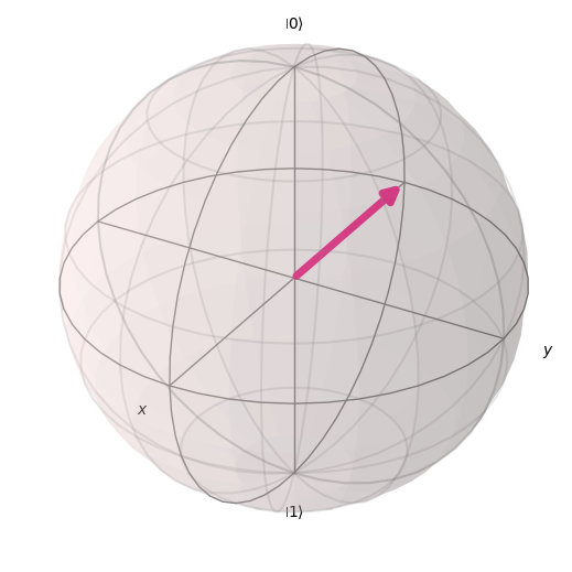
Using Qiskit, we plot the state \(\ket{-}\) in Cartesian and polar coordinates.
[8]:
# cartesian coordinates
plot_bloch_vector([-1, 0, 0], coord_type='cartesian')
[8]:

[9]:
# polar coordinates
plot_bloch_vector([1, -np.pi/2, 0], coord_type='spherical')
[9]:
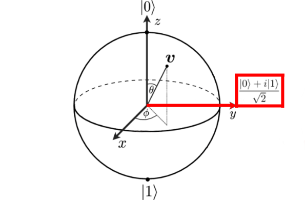
4. Y-Basis States
\(\ket{+i}\) and \(\ket{-i}\) are states located on the \(y\)-axis of the Bloch Sphere.
4.1 \(\ket{+i}\)
The \(\ket{+i}\) state lies on the positive \(y\)-axis, and is defined as:
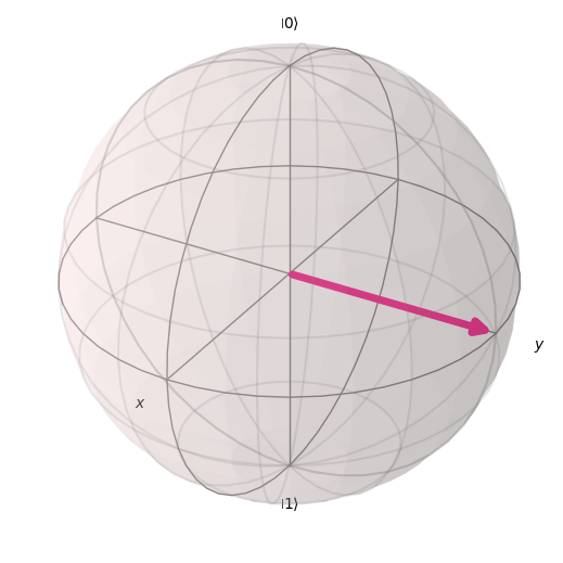
Using Qiskit, we plot the state \(\ket{+i}\) in Cartesian and polar coordinates.
[10]:
# cartesian coordinates
plot_bloch_vector([0, 1, 0], coord_type='cartesian')
[10]:

[11]:
# polar coordinates
plot_bloch_vector([1, np.pi/2, np.pi/2], coord_type='spherical')
[11]:
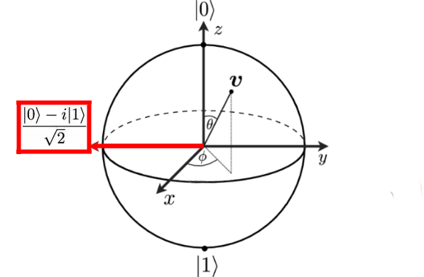
4.2 \(\ket{-i}\)
The \(\ket{-i}\) state lies on the negative \(y\)-axis, and is defined as:
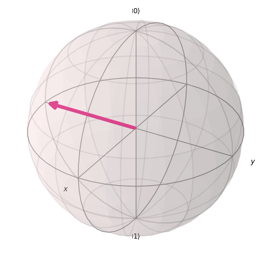
Using Qiskit, we plot the state \(\ket{-i}\) in Cartesian and polar coordinates.
[12]:
# cartesian coordinates
plot_bloch_vector([0, -1, 0], coord_type='cartesian')
[12]:
[13]:
# polar coordinates
plot_bloch_vector([1, -np.pi/2, np.pi/2], coord_type='spherical')
[13]:
